Contents

Introduction

The problem of chemical species transport in OpenWAM is solved including two possibilities:

A simplified transport model where only fresh air and burnt gas are considered as chemical species
An exhaustive transport model where the most important chemical species are taken into consideration: N₂, O₂, H₂O, CO₂, C (soot), H_xC_y, NO_x and CO.

In both cases, the transport of the fuel (diesel or petrol) is optional. If the user decides not transport the fuel, its mass fraction is included in the mass fraction of non-burnt hydrocarbons (H_xC_y) at exhaust valve opening.

Independently the use of the simplified or the exhaustive option, OpenWAM also includes the possibility of the transport of an specific chemical specie called EGR. This chemical specie, that is completely independent of any other chemical species calculation, allows the knowledge of the mass fraction of exhaust gases at any location and any time step. Therefore it is interesting for EGR transport and dispersion studies.

Chemical species transport model in 1D elements

OpenWAM is able to transport chemical species along the different elements of the engine. The calculation is performed including the mass fraction conservation equation to the governing equations system. In ducts, the solution of chemical species transport requires the addition of $n-1$ mass fraction conservation equations, where $n$ is the number of chemical species advected. The vectorial equation for chemical species transport is written as:

(1) $\begin{equation*} \frac{\partial \left( \rho \mathbf{Y} \right)}{\partial t}+\frac{\partial \left( \rho u\mathbf{Y} \right)}{\partial x}+\frac{\rho u\mathbf{Y}}{F}\frac{dF}{dx}=0 \end{equation*}$

where $\rho$ is the gas density, $u$ the gas velocity, $F$ represents the cross section area and $\mathbf{Y}$ is a vector composed by the mass fraction of $n-1$ different chemical species, from the total of $n$ species. The mass fraction of the last chemical specie is agree with the continuity equation and is given the equation of compatibility 1.

(2) $\begin{equation*} Y_{n}=1-\sum\limits_{j=0}^{n-1}{Y_{j}} \end{equation*}$

In equation 1 it is considered only the transport by convective phenomena. The term describing the diffusion between chemical species has been not included due to the fact that is negligible in comparison with the transport velocity inside ducts of internal combustion engines.

Considering the transport of chemical species along the ducts, the conservation equations system for perfect gas in conservative vectorial form is:

(3) $\begin{equation*} \begin{align} & \text{W}\left( x,t \right)=\left[ \begin{matrix} \rho F \\ \rho uF \\ F\left( \rho \frac{u^{2}}{2}+\frac{p}{\gamma -1} \right) \\ \rho S\mathbf{Y} \\ \end{matrix} \right]\text{ F}\left( \text{W} \right)=\left[ \begin{matrix} \rho uF \\ \left( \rho u^{2}+p \right)F \\ uF\left( \rho \frac{u^{2}}{2}+\frac{\gamma p}{\gamma -1} \right) \\ \rho uS\mathbf{Y} \\ \end{matrix} \right] \\ & \text{C}_{1}\left( x,\text{W} \right)=\left[ \begin{matrix} 0 \\ -p\frac{dF}{dx} \\ 0 \\ 0 \\ \end{matrix} \right]\text{C}_{2}\left( \text{W} \right)=\left[ \begin{matrix} 0 \\ g\rho F \\ -q\rho F \\ 0 \\ \end{matrix} \right] \\ \end{align} \end{equation*}$

Numerical methods adaptation to chemical species transport

The solution of equation system presented in 3 need the corresponding adaptation of the finitte difference numerical methods applied for duct solution in OpenWAM.

The symetrical second order Lax-Wendroff method of two steps needs a simple adaptation. The $n-1$ equations of chemical transport are discretised in the same way that the mass conservation equation. Only it has to take into account the both the solution and flux terms are multiplied by the mass fraction of chemical specie $i$ , $Y_i$ .
In the case of the TVD scheme of Sweby´s flux limiter, it has to consider that the vectorial version of the method calculates the Jacobian matrix of the governing equaitions system. The inclusion of the chemical species conservation does not provide new eigenvalues to the equations system. Therefore, it would be not possible to obtain the matrix $P^{-1}$ . In this way, the proposed solution consists in the use of the vectorial TVD solution for mass, momentum and energy conservation equations and the use of the scalar TVD version for the solution of every of the chemical species conservation equations.

Chemical species transport in 0D elements

The 0D elements are those engine elements with the ability to accumulate flow at the time the thermal-fluid-dynamic properties can be considered constant in all the volume every instant of calculation. Among these elements fall into the engine, the turbine, well-defined volumes in manifolds, intercoolers or mufflers, etc.

The 0D elements are solved as open systems by means of the application of a filling and emptying model. If the transport of chemical species is not considered, the filling and emptying models only need the application of two equations. The first equation is the mass conservation equation in open systems:

(4) $\begin{equation*} d m =\left(\sum{\dot{m}_{in}}-\sum{\dot{m}_{out}}\right)dt \end{equation*}$

In 4 $m$ is the mass of flow inside the element and $\dot{m}_{i}$ represents the mass flow entering or leaving the element through connection $i$ with other engine elements (1D or 0D).

The second of the equations is the First Principle of Thermodynamics applied to open systems:

(5) $\begin{equation*} d\left( me \right)=\delta q+\delta w+\sum{\left( h_{in}+\frac{u_{in}^{2}}{2} \right)d\dot{m}_{in}}-\sum{\left( h_{out}+\frac{u_{out}^{2}}{2} \right)d\dot{m}_{out}} \end{equation*}$

where $e$ represents the specific internal energy of the gas in the 0D element, $q$ is the heat transfer to/from the 0D element, $w$ is the mechanical work and $h$ and $u$ are the specific enthalpy and velocity of the flow (entering or leaving the volume).

The solution of the system composed by 4 and 5, together the state equation, provides the new thermodynamic conditions inside the 0D element in the last calculation time.

From the point of view of the solution, the inclusion of the chemical species modelling in the 0D elements involves:

The addition of as many mass conservation equations as chemical species transported minus one. It is to say, the mass fraction is $n-1$ chemical species will be calculated according to 6:
(6) $\begin{equation*} \Delta m_{Y_{j}}=\sum\limits_{i}{\dot{m}{}_{i}Y_{j}_{CC_{i}}\Delta t}\end{equation*}$

where $m_{Y_{j}}$ is the mass of chemical specie $j$ inside the 0D element and $Y_{j}_{CC_{i}$ is the mass fraction of chemical specie $j$ entering or leaving the 0D element trough the boundary condition $i$ . In this way, the mass fraction of specie $j$ at calculation time $t+\Delta t$ will be:

(7) $\begin{equation*} Y_{j}=\frac{m_{Y_{j}}+\Delta m_{Y_{j}}}{m+\Delta m} \end{equation*}$

The mass fraction of specie $n$ is given by equation 7, as in 1D elements.
In the case of the cylinder, where the combustion process takes place, there are two possibilities for the calculation of the chemical species conversion. In first place, it can be used the predictive combustion model ACT. This model, from the gas composition and thermodynamic properties inside the cylinder at inlet valve closing, provides not only the heat release law but also the gas composition at the exhaust valve opening. The second possibility for the combustion simulation is the use of Wiebe´s functions to define the heat release law. In this way, from this information OpenWAM gets the instantaneous gas composition by solving the stequiometrical balance of the fuel oxidation.

Chemical species transport in boundary conditions

The inclusion of chemical species transport in the model through boundary conditions does not mean any modification to the calculation process of the departure point of the characteristic lines or the flow path line. However, the value of the characteristics and the entropy level at the end of the duct is modified when the flow is considered a non-perfect gas as function of the composition and the temperature. For that reason, it is needed consider that:

The chemical species are transported from point $(y,t)$ at to the end of the duct ( $(x_n,t+\Delta t)$ if the end is the right one and $(x_0,t+\Delta t)$ if the end is the left one) through the flow path lines, which determines the path of the flow between both points.

The most widespread derivation of the Method of the Characteristics is based on the hypothesis that the flow is a perfect gas. This is the derivation adopted in OpenWAM. The derivation of the Method of the Characteristics involves higher difficulty for the calculation of the boundary conditions. Therefore, as most authors do, the gas properties are calculated as function of the composition and temperature at time $t$ , both at point $(y,t)$ and the boundary condition itself, for its solution at calculation time $t+\Delta t$ .

Gas properties variation with composition and temperature

Although there are several possibilities to calculate the properties of the gas to be applied on the solution of the governing equations system between the calculation times $t$ and $t+\Delta t$ , it is taken the proposal of . This solution consists in assuming that the values of the gas properties are constant during the time-step $\Delta t$ and in the spatial mesh size in which the problem is being solving, $\Delta x$ . Once the value of the temperature and the composition are known in the following calculation time it is possible to calculate again the gas properties.
The evaluation of the gas properties is based on the instantaneous and local temperature and composition. It is also needed to consider the properties of every chemical species composing the gas. Here it is need to distinguish between the calculation when OpenWAM applies the exhaustive transport model or the simplified transport model for chemical species.
With regard to the exhaustive transport model, it consists of 9 chemical species, listed in Figure 1. Additionally, as explained in the introduction, the fuel (diesel or petrol) can be also transported. The particulates are modelled as solid carbon, assuming that there is not any relative momentum between the particulates and the gas flow. This hypothesis is consistent with the results shown by Foster et al. in .

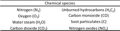
Figure 1. Chemical species considered in the exhaustive calculation.

For simplicity sake, the model calculates the gas properties only as funcion of NO₂, O₂, CO₂, H₂O and Argon content. Regarding the mass fraction of pollutants, it is added to the mass fraction of N₂ for gas properties calculation due to the fact it is negligible in comparison with the others. In the case of the Argon, it is a chemical specie that is not included in the transpor model but consider with a constant mass fraction of 0.012 in the calculation of gas properties at any element and location. This mass fraction is substracted from N₂ mass fraction.

Under these considerations, the specific gas constant if givin by 8:

(8) $\begin{equation*} R_{g} = R_{N_2 } Y_{N_2 } + R_{O_2 } Y_{O_2 } + R_{Ar} Y_{Ar} + R_{H_2 O} Y_{H_2 O} + R_{CO_2 } Y_{CO_2 } \end{equation*}$

The values of the gas constant for every chemical species are shown in Figure 2.

Figure 2. Specific gas constant for every chemical specie.

On the other hand, the calculation of the specific heat capacity at constant pressure is obtained according to 9:

(9) $\begin{equation*} c_{p_g } = c_{p_{N_2 } } Y_{N_2 } + c_{p_{O_2 } } Y_{O_2 } + c_{p_{Ar} } Y_{Ar} + c_{p_{H_2 O} } Y_{H_2 O} + c_{p_{CO_2 } } Y_{CO_2 } \end{equation*}$

The specific heat capacity of every chemical species is calculated as function of the gas temperature with the correlations proposed by JANAF . These correlations are applied inside the temperature range between 0 K and 6000 K. This database is used in other wave action models , in the combustion prediction model ACT coupled with OpenWAM and in the diagnostic combustion model developed also at CMT Motores Térmicos . According to JANAF´s correlation, the specific heat capacity of any chemical specie is given by 10

(10) $\begin{equation*} c_p \left( T \right) = R\left( {a_1 T^{0.5} + a_2 + a_3 T^{ - 0.5} + a_4 T^{ - 1} + a_5 T^{ - 1.5} } \right) \end{equation*}$

The coefficients a_i from 10 are detailed in Figure 3 for every chemical specie considered in calculations.

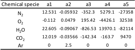
Figure 3. Coefficients in the correlation of specific heat transfer cp(T) for every chemical specie considered in the calculation of the wave action model OpenWAM.

When the simplified model for chemical species transport is applied, OpenWAM only considers (as standard) fresh air and the products of the combustion. Like for the case of the exhaustive model, fuel can be also advected. In such a way, the specific gas constant is given by equation 11:

(11) $\begin{equation*} R_{g}=R_{b}Y_{b}+R_{air}\left( 1-Y_{b}-Y_{H_{2}O} \right)+R_{H_{2}O}Y_{H_{2}O} \end{equation*}$

The values of the gas constant are 287 J/kgK for fresh (dry) air, 285.4 J/kgK for products of the combustion and 461.398 J/kgK for water steam. It has to be noted that the inclusion of water is made to take into account the humidity in fresh air. For simplicity sake it is taken a constant content of 1.64% of mass fraction of water steam in fresh air (it corresponds to 50% of relative humidity at 25ºC).

With regard to the specifi heat capacity of the flow (at constant volume), it is given by equation ??:

(12) $\begin{equation*} c_{v}_{_{g}}=c_{v}_{_{b}}Y_{b}+c_{v}_{_{air}}\left( 1-Y_{b}-Y_{H_{2}O} \right)+c_{v}_{_{H_{2}O}}Y_{H_{2}O} \end{equation*}$

In this case, the specific heat capacity of the steam water is given by the use of JANAF correlation (calculation of c_p minus R). The correlation for the specific heat capacity of fresh (dry) air and products of the combustion are given by:

(13) $\begin{equation*} c_{v}_{_{b}}=614.154+0.43045T-0.0001125T^{2}+8.979e-9T^{3} \end{equation*}$

(14) $\begin{equation*} c_{v}_{_{air}}=-10.4199T^{0.5}+2522.88-62227.1T^{-0.5}+917124.4T^{-1}-4174852.6T^{-1.5} \end{equation*}$

Every coefficient is obtained taken into account the composition of the fresh (dry) air (mass fraction of every chemical species) and its JANAF correlation for specific heat capacity calculation.

Chemical Species Transport