Wiebe’s function for combustion simulation

The model used in Openwam is based on the use of Wiebe’s functions. The Wiebe´s functions simulate pilot, premixed, diffusion and late combustion phases.
The mathematical expression of the rate of heat release given by a Wiebe´s function is,

(1) $\begin{align*} HRL=\beta_{0}[1-e^{[-c_{0}(\frac{\alpha-\alpha_{0}}{\Delta \alpha_{0}})^{(m_{0}+1)}]}]+\beta_{1}[1-e^{[-c_{1}(\frac{\alpha-\alpha_{1}}{\Delta \alpha_{1}})^{(m_{1}+1)}]}]+ \\ \beta_{2}[1-e^{[-c_{2}(\frac{\alpha-\alpha_{2}}{\Delta \alpha_{2}})^{(m_{2}+1)}]}]+\beta_{3}[1-e^{[-c_{3}(\frac{\alpha-\alpha_{3}}{\Delta \alpha_{3}})^{(m_{3}+1)}]}] \end{align*}$

which is the derivative of the heat release:

(2) $\begin{align*} RoHR=[\frac{c_{0}(m_{0}+1)}{\Delta\alpha_{0}}(\frac{\alpha-\alpha_{00}}{\Delta \alpha_{0}})^{m_{0}}e^{[-c_{0}(\frac{\alpha-\alpha_{00}}{\Delta \alpha_{0}})^{(m_{0}+1)}]}\beta_{0}]+ \\ + [\frac{c_{1}(m_{1}+1)}{\Delta\alpha_{1}}(\frac{\alpha-\alpha_{01}}{\Delta \alpha_{1}})^{m_{1}}e^{[-c_{1}(\frac{\alpha-\alpha_{01}}{\Delta \alpha_{1}})^{(m_{1}+1)}]}\beta_{1}]+ \\ + [\frac{c_{2}(m_{2}+1)}{\Delta\alpha_{2}}(\frac{\alpha-\alpha_{02}}{\Delta \alpha_{2}})^{m_{2}}e^{[-c_{2}(\frac{\alpha-\alpha_{02}}{\Delta \alpha_{2}})^{(m_{2}+1)}]}\beta_{2}]+ \\ + [\frac{c_{3}(m_{3}+1)}{\Delta\alpha_{3}}(\frac{\alpha-\alpha_{03}}{\Delta \alpha_{3}})^{m_{3}}e^{[-c_{3}(\frac{\alpha-\alpha_{03}}{\Delta \alpha_{3}})^{(m_{3}+1)}]}\beta_{3}] \end{align*}$

In this two equations, $\alpha$ is the crank angle; $\Delta\alpha$ is the duration of the combustion phase $i$ (premixed, diffusion or late combustion); $\alpha_{0i}$ is the crank angle at which the combustion phase $i$ stars; $\beta$ represents the proportion of the combustion phase $i$ with regard to the whole combustion. Hence, its value varies between 0 and 1; $C_i$ represents the modulation parameter that controls what percentage of fuel injected is burnt within the combustion duration; and $m_i$ is the shape parameter that controls the gradient of the combustion phase $i$ .

RoHR are normalised by dividing the heat release energy by the injected fuel energy. As a consequence, the value of the area under the function is equal to 1. The reference RoHR versus crank angle comes from the combustion diagnostic code .

HRL interpolation for non-defined operating point

In some cases, mainly when in the modelling of transient operation, it is needed to predict the HRL for the engine conditions so that the prediction of the Wiebe’s functions to simulate the combustion process becomes critical. The model applied in OpenWAM proposes the use of a simple technique to interpolate the RoHR versus crank angle value from an engine database of empirical results. The proposed interpolation model is supported by an engine database that represents the engine transient operation range homogeneously. It is composed by a set of parametrized RoHRs, which are obtained by using the criteria describe in . Every RoHR is associated to the following average cycle variables, which are going to be referred as interpolation parameters:

Air mass.
Fuel mass.
Engine speed.
Boost pressure.
Charge air temperature.
Start of injection (SOI).
Air to fuel ratio.
EGR mass.
Charged air density.

The interpolation model takes into account the necessity of distinguishing between the interpolation of the combustion beginning, on the one hand, and the interpolation of the RoHR values, on the other hand. The interpolation technique is based on weighted linear interpolation between several RoHR similar to that described in . By inheriting the philosophy described by , the interpolation model calculates the distance from the current running point to the measured ones in a n-dimensional space (composed by the interpolation parameters) by applying Equation 3.

(3) $\begin{equation*}d_{j}= \sqrt{\sum_{i=0}^{n-1}\left ( \frac{p_{i}-p_{i_{j}}}{p_{imax}} \right )^{2}}\end{equation*}$

where $d_j$ is the distance from the $j$ operating point of the database to the current one, $n$ is the number of parameters to be considered and $p$ represents the value of every the parameter. Every parameter, both running and measured, is normalised to its corresponding maximum within the engine database. An example of distance calculation for a three-dimensional space is shown in Figure 1.

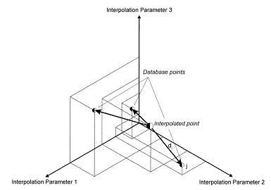
Figure 1. Distance calculation in a three dimentional space for RoHR determination

The distance of every operating mode in the database to the current running point indicates the relative weight of every RoHR in the final interpolated RoHR. However, the differences among these distances are too slight even though between operating points in the database which are very close or very far away from the current running point respectively. In order to magnify these differences and calculate the weight of every RoHR composing the database, the distance previously calculated is corrected by means of the following exponent:

(4) $\begin{equation*}e=4+\frac{2}{d_{j}}\end{equation*}$

Thus, the weighted distance from every measured operating point composing the database to the current one is calculated as:

(5) $\begin{equation*}d_{weighted_{j}}=\left ( \sqrt{\sum_{i=0}^{n-1}\left ( \frac{p_{i}-p_{i_{j}}}{p_{imax}} \right )^{2}} \right)^{e}\end{equation*}$

Due to the fact that both combustion beginning, αcb, and RoHR value are interpolated separately, the weighted distances are termed as $d_{weighted_{j}}$ and $RoHR_{weighted_{j}}$ respectively.
The beginning of the combustion interpolation requires information related to the SOI and additional variables related to the time delay associated to the combustion. The lack of generality of time delay models, due to their dependence on ambient geometrical conditions, has led to propose a set of basic interpolation parameters that simulate the trend of the time delay. Thus, the beginning of the combustion, which is only calculated once per cycle, is performed by weighting the distance in a n-dimensional space conformed by:

Start of injection (SOI),
Engine speed,
Air to fuel ratio,
EGR mass,
Charged air density,

whose influence on the combustion is analysed in literature . The use of this set of parameters manages the intrinsic information regarding the time delay. The combustion beginning is simulated in an accurate way according to Equation 6.

(6) $\begin{equation*}\alpha_{cb}=\frac{\sum_{j=0}^{m-1}\frac{\alpha _{cb_{j}}}{d_{cb_{weighted_{j}}}}}{\sum_{j=0}^{m-1}\frac{1}{d_{cb_{weighted_{j}}}}}\end{equation*}$

On the other hand, the n-dimensional space to carry out the calculation of the weighted distance for the interpolation of RoHR values is defined by:

Air mass.
EGR mass.
Fuel mass.
Engine speed.
Boost pressure.
Charge air temperature.

Traditionally, in the interpolation techniques , the air mass, the fuel mass and the engine speed have been the only weighted variables. Nevertheless, the increasing trends in boosting pressure and EGR rates make these two variables necessary for guaranteeing a certain level of accuracy, due to the influence of these parameters on diesel combustion. RoHR values are interpolatedevery time-step of the gas dynamic code and at every cylinder of the simulated engine. A primordial requirement to reach a correct simulation of the RoHR is that each RoHR in the database has to be referenced to the combustion beginning of the current running point. Thus, it is calculated the transfer angle to be applied to each of the Wiebe´s functions of the RoHR $j$ in the database, as is shown in Equation 7.

(7) $\begin{equation*} \Delta \alpha _{transfer_{j}}=\alpha_{cb}-\alpha_{cb_{j}} \end{equation*}$

Once each RoHR in the database is referred to the angle $\alpha_{cb}$ , the value of the RoHR versus the crank angle is calculated as

(8) $\begin{equation*} RoHR(\alpha)=\frac{\sum_{j=0}^{m-1}\frac{RoHR(\alpha){}_{j}}{d_{RoHR_{weighted_{j}}}}}{\sum_{j=0}^{m-1}\frac{\1}{d_{RoHR_{weighted_{j}}}}} \end{equation*}$

Four Wiebes simulation

Wiebe’s function for combustion simulation

HRL interpolation for non-defined operating point

Login

Search Forums