Introduction

The wave action models carry out the thermal- and fluid-dynamics calculation in each part of the engine. The different elements of the engine are represented by 0D, 1D and boundary conditions. 1D elements have a axially spatial mesh that establishes the calculation nodes in which, the conservation equations system is solved. The spatial meshing is imposed by the user, who would have adopted this solution in order to obtain an appropriate balance between accuracy, reliability and computational cost . This decision will determine the spatial structure of the calculation. It still remains to define the structure of the calculation which manages the temporary advance of the wave action model WAM. This definition has to be closely linked to the stability criteria applied to each element of the model.From it application, it is obtained the maximum temporary increase that it may be imposed to avoid numerical stability problems.

In the 1D elements, the stability condition applied is the Courant-Friedrichs-Lewy criterion, commonly known as CFL stability criterion . This criterion imposes that the information, in the form of disturbances or waves, cannot travel more than one mesh length (distance between two nodes) in one calculation time increment. Therefore, for each compute node it will be necessary:

$\Delta t\leq \nu \frac {\Delta x}{c^{p}}$

The parameter $\nu$ is known as the Courant, or CFL, number and its value is in the range [0,1]. $c^{p}$ represents the largest wave speed present in the node at time level $p$ . In the practice, all nodes in a duct are solved with the same time-step, therefore the last equation is rewritten as:

$\Delta t=\nu \frac {\Delta x}{c^{p}_{max}}$

Now, $c^{p}$ represents the largest wave speed present in the entire solution domain at time level $p$ . From the expression of the CFL stability criterion, it is deduced that, regarding the computational cost will be most efficient when the value of this parameter is close to 1.In any case, the reduction of the spatial mesh in the ducts increases computational cost. It is due to the increase of the calculation nodes and how it is shown in the CFL criterion, the time increase with which it is possible to solve the conservation equations also is reduced.This means that to achieve the ending of execution the will be necessary to resolve a higher number of times the system of conservation equations.

In the case of 0D elements, the stability criterion applied is related to prevent the complete emptying during the step.

<!–-nextpage–->

Common Time Discretization

The calculation methodology of the wave action models arises from the way in which the results of the application of stability criteria to 1D and 0D elements is managed. The most extended calculation structure due to it simplicity in the wave models is the Common Time Discretization (CTD),and its diagram is represented in Figure 1. In the CTD structure calculation, the most restrictive stability criterion is applied as global integration step for all elements of the model. For this reason all the model elements are calculated using the minimum time-step. Thus, the calculation stability is ensured.

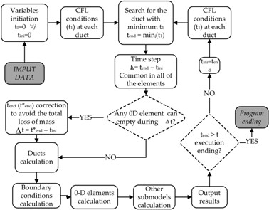
Figure 1. Flow chart of the CTD programme layout

First, the model variables initialization are performed ( $t_0 = 0$ for all the ducts and elements of the model), as well as the initial time step, $t_{ini} = 0$ . After applying the CFL criterion for all ducts of the engine, the maximum time $t_1$ to each of them could move is obtained. Then, the duct with the minimum time $t_1$ is searched, and this is the maximum time with which the model can progress in this time step $t_{end} = t_1$ . Thus, the common time step will be:

$\Delta t=t_{end}-t_{ini}$

It is necessary to check that in this time step, the stability criterion is carried out for all the 0D elements. Otherwise, it would be necessary the time step correction to achieve this more restrictive condition. Once the verification or it corresponding correction (if it is necessary) are completed, the thermo- and fluid-dynamics conditions in the ducts, boundary conditions and 0D elements are calculated with the common time step. Finally, other sub-models such as the VGT position or the EGR valve are calculated as weel as the outlet results.With this, all calculations corresponding to the time step are solved and then it is only necessary to check if the program is ended. Otherwise, the calculation of the next time step is started.
From the point of view of the programming control structure, the CTD calculation is very simple, but it supposes, from the CTD diagram, an important computational cost penalty. It is due the fact that most common case is that there are ducts with different spatial mesh (it is shown in Figure2). According to the CFL criterion, the ducts with a lower meshing could be calculated with a higher time step, and therefore less number of times. The objective is the use of the understanding of this phenomenon in order to optimize the calculation structure of the wave action models and contribute to decreasing the computational cost without the loss of the precision and accuracy.

Figure 2. Objectives of accuracy and computational effort trade-off for the new calculation methodology and final Time-marching of Common Time Discretization.

Independent time discretization

With the need to optimize the calculation structure of the wave action models to reduce the computational cost, it is proposed a computational structure in which each elements of the 1D model are calculated with the temporary increase resulting from application of their own CFL stability criterion. Thus, when it is essential to introduce an exceptionally low mesh in some duct, it will be caught up the objective of achieving higher local precision at the expense of increasing the local computational cost, without affecting the rest of the simulated elements. With this philosophy of computation, which has been called Independent Temporal Discretization and whose acronym is ITD, it is possible to achieve the target. The same calculation example in Figure 2 but resolved with the computational structure ITD, Figure 3, show that it is possible to reduce drastically the number of times that the ducts with a higher spatial mesh are solved.

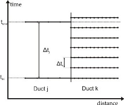
Figure 3. Example of the ITD calculation structure where it is shown the reduction of calculation performed in a duct with higher mesh.

However, as is shown in Figure 3, when the time step calculation is carried out in the duct j it is not possible to assure that the duct k is in the same time instant. The characteristics of the ITD calculation structure involves that the flowchart is more complex and requires more attention than the CTD structure. In Figure 4 it is shown the ITD flow chart. In the ITD structure calculation a loop is defined in which is resolved with a specific temporary increase the conservation equation system in the 1D elements, and the 0D elements and boundary conditions connected to them. This loop is included inside a main loop that controls the well-running of the execution.

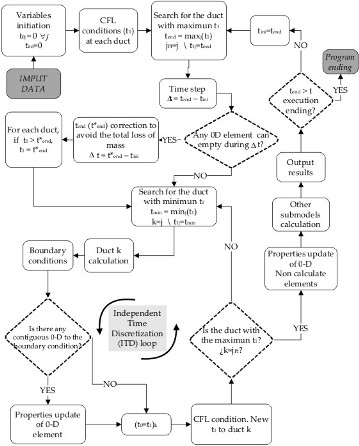
Figure 4. Flowchart of the ITD programme layout.

First, the initialization of all variables are carried out and the variables $t_0$ and $t_1$ are assigned to each duct. $t_0$ is referred to an initial instant calculation and $t_1$ is the specific calculation instant until that the calculation of each duct can progress according to the CFL stability criterion.On the other hand $t_{ini}$ and $t_{end}$ , that represent the initial and final calculation time after a global time step of the model, are defined. Further, the duct whose $t_1$ is maximum is searched, which defines tend. Once tend is known, the global time-step is set as:

(1) $\begin{equation*} \Delta t=t_{end}-t_{ini} \end{equation*}$

During the global time-step every engine element will be calculated one time at least. For each element, the global time-step will divide in many specific time-steps according to its own criteria. The global time-step defined in equation 1 is modified if any 0D element would need a more restrictive time step to fulfill its stability criteria. If this would be necessary, tend value came to be $t_{end}*$ .The same happens in each duct in which the value of $t_1$ is higher than $t_{end}*$ . With this, the global and the specifics time-step will be corrected. Next, the governing equations are solved in the ducts whose $t_1$ is minimum. Furthermore, its boundary conditions are solved as well, but it must be taken into account that the rest of the engine elements are at a different calculation time. If there is any 0D element contiguous to this duct, its thermodynamic properties are calculated solving mass and energy balance from the results got from the boundary condition solution. In this case, it is considered that any other duct connected the duct keeps its thermodynamic properties and mass flow constant since the last time in which this duct was calculated. Finally, the next $t_1$ value for the current duct is set by applying the CFL stability criterion. These calculation are carried out as many times as required until the duct calculated sets the global time-step. In this moment the ITD loop will finish, and the calculation of the other submodels and the result output are carried out. Also the temporary upgrade of those 0D elements which have not been calculated during the time-step for staying closed is performed. This solution helps to reduces the computational cost. Finally the programme checks if the execution has ended. If the programme ending has not been reached, the duct whose $t_1$ is maximum is searched in order to get the new global time-step and the ITD loop begins again. This iterative process is carried out until the calculation end is reached.

Independent time discretization in boundary conditions.

The use of the ITD calculation methodology requires the adaptation of the boundary conditions resolution. On this matter, three kinds of boundary conditions have to be distinguished depending on the type of engine components that the boundary condition connects:

Extreme boundary conditions of 1D elements. This group includes the boundary conditions that represent the extremes of closed ducts, anechoic or open to a particular atmosphere.Includes other specific cases where the imposition of a pressure pulse is the most important.Its resolution has not difference on CTD structure calculation.
Boundary conditions of 1D connected to 0D elements. There is not any difference in the way the boundary condition is solved with regard to the CTD programme layout. However, it is necessary take into account how is affected the resolution of mass and energy balances that determine the thermodynamic conditions inside the 0D elements. As previously stated, every time a contiguous duct is solved, the 0D element has to be updated to the current calculation time. In order to carry out the energy and mass conservation balances inside the 0D element, every duct end connected to the 0D element has to be considered. This fact leads to take into account last calculated results for every boundary condition by assuming that the information is frozen since last time they all were calculated until the current calculation time.
Boundary conditions between 1D elements. In this case, when the boundary condition is solved it must be considered that each duct connected to the boundary condition is at a different calculation time. This situation is represented in Figure 5, which shows the obtaining the characteristics lines and entropy level between two ducts. Every point represented a node of the duct and the gas velocity is assumed from right to left in the ducts. In this situation, the duct k is being solved. Its calculation time is $t_{0k}$ and the calculation has to advance until the instant $t_{1k}$ . For that, the thermo-fluid-dynamic properties of the duct $j$ are available at the calculation time $t_{0j}$ .

In order to solve the boundary condition, the origin of the three characteristic and stream lines has to be found, so all of them pass through the extreme node of duct k in the calculation time $t_{1k}$ . Due to the fact that each duct is in different calculation time, two different time-steps need to be distinguished: $\Delta t_k$ and $\Delta t_{jk}$

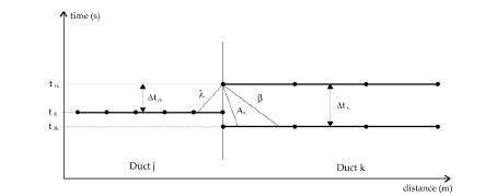
Figure 5. Solution of the boundary condition for a junction of two ducts.

Calculation Methodology

Introduction

Common Time Discretization

Independent time discretization

Independent time discretization in boundary conditions.

References

Login

Search Forums